logo image

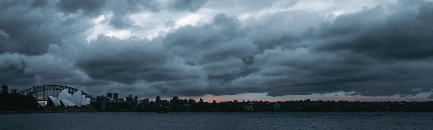
Still ranked within the top three largest insured loss events in Australia’s history, it has now been twenty years since a hailstorm shattered roofs across the eastern suburbs of Sydney on April 14, 1999. And recent events continue to show the significant risk posed by severe hailstorms – on December 20, 2018, Sydney was hit by “…the worst hailstorm in twenty years” according to the Australia Bureau of Meteorology. On the anniversary of the 1999 storm, we look at both these events and discuss the return period of significant hail losses in Sydney.

For the 1999 event, the large hail associated with the storm damaged 24,000 homes and 70,000 automobiles along its path. There has been much written about the 1999 event, and in 2009 RMS published a detailed 10-year retrospective, but in short, this storm was unusual for several reasons:

  • April 14 was outside of the normal storm season which tends to focus around September through to March
  • The storm had hit late in the day, at 8 p.m. local time; most hit during the mid to late afternoon
  • The size of the hailstones was very large, described at the time as “… cricket-ball, melon, or grapefruit sized…” and up to 12 centimeters (4.7 inches) wide.


Realizing the Return Period

What would the losses from the 1999 storm look like now? RMS has previously simulated the 1999 event using techniques from the RMS Australia Severe Convective Storm model to apply spatial noise to the size of the hail reaching the ground. We computed ground-up losses to our Industry Exposure Database for each of 200 realizations of the event and generated a distribution of losses which has an expected loss of AU$4 billion (US$2.87 billion). The latest trended loss from the Insurance Council of Australia (ICA) is AU$5.6 billion (US$4 billion) which fits comfortably inside our loss range.

Trending losses is far more complicated than it sounds as uncertainties compound over time. We have not trended the loss, we have run multiple realizations of the event over today’s exposure.

It is important to note the range of these losses from these realizations. Large hail can fall in the harbor, on golf courses and parks without causing loss or it can fall just a few hundred meters away on tiled roofs with very expensive consequences. This variability explains why it is so difficult to estimate losses accurately immediately after an event. Further, it demonstrates how a “repeat of the storm” is not the same as a “repeat of the loss”.

Since 1999, the market has debated the return period of the loss from this event. Ten years ago in our retrospective, we concluded the event was not a “once-in-a-lifetime” event from a hazard perspective and we agreed with other authors the loss return period was “decades” and certainly “less than 100 years”. Such estimates were supported by other historical events, notably the New Year’s Day hailstorm of 1947. Today we have another significant historical datapoint for comparison.

Sydney Hailstorm 2018

On December 20, 2018, Sydney was hit by another band of severe storms. Perhaps being so close to the Christmas holidays, the event escaped the intense media attention it would otherwise have garnered. Smashing roofs and windows, just two days after the storm, the ICA declared the incident a “catastrophe” and reported the industry had already received 25,000 claims. A fuller summary of the event written a week after the event can be found here.

What did the losses look like? We simulated 200 realizations of the December 2018 event on the RMS Australia Industry Exposure Database, and the expected loss is approximately AU$2.2 billion (US$1.57 billion) with a range from under AU$1 billion to over AU$4 billion.

Other sources including the three-month progress report from PERILs at AU$633 million (excluding motor) and press releases from large primaries, it is almost certain final losses will exceed AU$1 billion. Some analysts expect losses to reach AU$2 billion, in line with the expected ground-up loss from our simple simulation.

As mentioned previously, the final loss from events such as these is very sensitive to exactly where the large hail fell, so it is important to consider the loss distribution and not simply the mean. It seems likely the expected loss from December 2018 will be roughly one-half of the losses from April 1999. It is also important to note the overlap in the loss distributions for the two storms. A “lucky” repeat of the April 1999 event would not cause as much loss as an “unlucky” repeat of the December 2018 storm.

Comparing the expected losses for 1999 and 2018 against our Industry Loss Curve confirms our hypotheses from ten years ago. The 1999 loss is large, but nowhere close to the maximum credible hail loss.

Sydney experiences losses of AU$1.5 billion every decade or two, as evidenced by the events in 1947, 1990, 1999 and 2018. With tiled roofs continuing to be popular in the city, these will continue to be damaged by large hail. And if Sydney-siders can therefore expect insured losses in excess of $1.5bn every decade or so, it is very likely that children at school in the city today will see at least one 1999-sized loss, or larger, in their lifetimes.

Analysis provided by Sanjna Sethi, Alpana Das and the RMS Noida Knowledge Center plus Rohit Mehta and Callum Higgins.

Share:
You May Also Like
Christchurch Earthquake 2011
November 12, 2020
Earthquake Insurance: Should California Be More Like New Zealand?
July 30, 2019
Should New Zealand Be Content with the New EQC Coverages and Caps?

The revised earthquake coverages and caps proposed by the New Zealand Earthquake Commission (EQC) came into law as planned on July 1, 2019. As noted in an RMS blog back in February, these well signaled changes – to increase the building coverage from NZ$100,000 to NZ$150,000 and remove the NZ$20,000 contents cover, only had a small effect on the gross average annual loss for both EQC and the private market. Swapping the first layer of contents exposure for a larger, higher layer of building exposure produced a result that was close to neutral. Examining the Exceedance Probability (EP) curve (see figure 1 below), the changes are small across all return periods. There are small increases in loss for the private market at short return periods (which produce the small increase in average annual loss reported earlier) but very little change at long return periods. Critically, the modeled gross 1000-year loss to the private market is essentially unchanged, meaning there are no implications with regards to the Reserve Bank of New Zealand (RBNZ) solvency requirements. Further, these EQC coverage changes are not expected to affect the peril balance driving trans-Tasman solvency considerations where both the RBNZ and Australian Prudential Regulation Authority (APRA) standards must be met.   Figure 1: New Zealand EQC and private market return period losses by residential occupancy under old and new EQC coveragesSo, is that the end of the story? Our model results are based on the RMS Industry Exposure Database (IED) so our conclusions rely on the data and assumptions used to estimate the total insured exposure in New Zealand. As we always say in RMS model guidance, our industry results should be used as a guide, but do not expect every individual portfolio to behave the same way. Whether or not swapping contents cover for an extra layer of buildings cover delivers a neutral result will be sensitive to the values and limits assigned to each coverage. So, how confident are we in our exposure estimates? An RMS IED is developed from the bottom-up, i.e. from building counts, floor areas and construction costs and then validated against local, regional and national macro-economic and demographic benchmarks. For buildings, there is a lot of information to work with, so we have high confidence in our estimated economic and insured building exposure. There is less information for other coverages, so we estimate those as ratios of the overall building exposure. The ratios for New Zealand are consistent with other similar markets around the world. Importantly in our IED, the contents replacement values are estimated, and we then assume the sums insured (the limits) are the same as the replacement values. There is an accompanying client reference guide available via RMS Owl that provides more details on our New Zealand IED methodology. Why do we need to estimate contents values? It is true, unlike residential buildings policies, contents policies have always had a specified sum insured. Those sums insured are the limits but how reliable are those figures as estimates of the replacement values? How much underinsurance is there and how has that been coded when models have been run? The recent changes to EQC are the third time since the Canterbury Earthquake Sequence (CES) in 2010/2011 that exposure values have been put under the spotlight. Immediately after the CES, underinsurance of commercial buildings combined with a lack of average in claims handling drove decisions to rebuild rather than repair. It is imperative model users recognize underinsurance when entering exposure into models or they will obtain unconservative results. The change from open-ended replacement policies for residential buildings to those based on sums insured was imposed on the New Zealand market by the global reinsurers in the years after the CES. This change forced insurers and homeowners to estimate actual replacement values. This is a deceptively difficult task for an individual building. There is no doubt that online calculators can be extremely useful tools – so long as it is understood that their precision is not to be mistaken for accuracy. Model users would be well advised to run sensitivity tests for underinsurance by scaling the specified sums insured to estimate replacement values lest they repeat the expensive lessons learned from commercial claims in Christchurch. Now, the removal of contents cover by the EQC is forcing the market to focus on estimating residential contents replacement values. While contents values are lower than building values, they are harder to estimate. It is logical the contents value should increase with the building value across a portfolio, but dwelling by dwelling, what is the contents value? How much does it cost to replace the fridge, the dining table, the food in the cupboard, all the children’s shoes and so on? It adds up – and faster than most homeowners realize. The public is both apathetic when in comes to investing time to take stock of their possessions and lightning fast with criticism on social media. Consequently, it may take many years until the industry accurately quantifies underinsurance for residential contents. Right now, though, individual insurers can test the sensitivity of their risk to this underinsurance by running different assumptions through the model. In this way they can put some bounds on the new contents risk they have received from the new EQC arrangements. Data quality is improving but no one should be content to stop improving now. The New Zealand market has seen a lot of changes since the CES in 2010/2011 and it is likely there are more changes to come.…

Michael Drayton
Michael Drayton

Michael Drayton has worked with RMS for over 20 years developing and supporting catastrophe models on a wide range of perils.

As a modeler based in London, he worked on the first generation of continent-wide models for European winter storms and the first basin-wide North Atlantic hurricane models.

He returned home to New Zealand in the early 2000's, modeled Australian cyclone risk and developed a high-resolution convective storm model.

Since the Canterbury Earthquake Sequence in 2010-2011 Michael has been the RMS liaison between model developers and local experts from many disciplines as well as insurers, regulators and government. He has an academic background in Civil Engineering and Applied Mathematics.

cta image

Need Help Managing Your Portfolio?

close button
Overlay Image
Video Title

Thank You

You’ll be contacted by an Moody's RMS specialist shortly.